Twin Neural Network Training with PyTorch and Fast.ai and its Deployment with TorchServe on Amazon SageMaker

September 15, 2022 By Mark Otto 0

A Twin Neural Network (commonly known as a Siamese Neural Network) makes predictions leveraging information from multiple sources. A common use case is taking multiple input data, such as two images, and predicting whether they belong to the same class, though its applications aren’t necessarily limited to computer vision or classification problems. In practice, however, artificial neural network training takes extensive and sophisticated effort. Fortunately, there are a variety of deep learning frameworks available to tackle training. One which stands out, Fast.ai, has become one of the most cutting-edge, open source, deep learning frameworks based on PyTorch. It provides a concise user interface and well designed, documented APIs, which empowers developers and machine learning practitioners to train models with productivity and flexibility.

For deployment, Amazon Web Services (AWS) developed TorchServe in partnership with Meta (previously, Facebook), which is a flexible and easy-to-use open source tool for serving PyTorch models. It removes the heavy lifting of deploying and serving PyTorch models with Kubernetes. With TorchServe, many features are out-of-the-box and they provide full flexibility of deploying trained PyTorch models at scale. In addition, Amazon SageMaker endpoint is a fully managed service that allows users to make real-time inferences via a REST API, which saves developers from managing their own server instances, load balancing, fault-tolerance, auto-scaling and model monitoring, etc. Amazon SageMaker endpoint supports industry level machine learning inference and graphics-intensive applications while being cost-effective.

In this post we demonstrate how to train a Twin Neural Network based on PyTorch and Fast.ai, and deploy it with TorchServe on Amazon SageMaker inference endpoint. For demonstration purposes, we build an interactive web application for users to upload images and make inferences from the trained and deployed model, based on Streamlit, which is an open source framework for data scientists to efficiently create interactive web-based data applications in pure Python.

All the code used in this document is available on GitHub.

Getting started with a PyTorch model trained with Fast.ai

In this section, we train a Fast.ai model that determines whether the pets in two images are of the same breed or not.

The first step is to install a Fast.ai package, which is covered in its GitHub repository.

If you’re using Anaconda then run:

conda install -c fastai -c pytorch -c anaconda fastai gh anaconda

…or if you’re using miniconda then run:

conda install -c fastai -c pytorch fastai

For other installation options, please refer to the Fast.ai documentation. The following materials are based on the documentation: “Tutorial – Using fastai on a custom new task“, with customisations specified below.

Model Architecture

For Twin Neural Networks, multiple input data sources are passed through an encoding neural network to generate their hyper-dimensional embedding vectors, which are concatenated before fed into a Fully Connected Network (FCN) for output, as shown in Fig. 1.

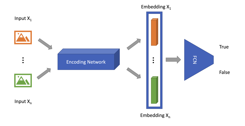
Fig. 1 — Twin neural network architecture.

Now that Fast.ai is installed, we can define this model architecture in pure PyTorch for Fast.ai training. Specifically, we will load the pre-trained encoding network from PyTorch, and define our customised FCN, before passing the images through both.

Encoding Network

For the encoding network, ResNet50 is used as an example with its pre-trained weights, and the last fully connected layer is removed to be replaced by our own FCN in the following step.

import torchvision.models as models
from torch.nn import ( Sequential,
) encoder = Sequential( *list( models.resnet50(pretrained=True).children() )[:-2] )

Fully Connected Network

This model consists of concatenated average and max pooling (according to Fast.ai), tensor flattening, batch normalisation, dropout, linear layers and activation functions. The output is a single vector of size 2 indicating if the input images are different or the same.

from torch.nn import ( AdaptiveAvgPool2d, AdaptiveMaxPool2d, Flatten, BatchNorm1d, Dropout, Linear, ReLU, Module, Sequential,
) class AdaptiveConcatPool2d(Module): "FastAI: Layer that concats `AdaptiveAvgPool2d` and `AdaptiveMaxPool2d`" def __init__(self, size=None): super().__init__() self.size = size or 1 self.ap = AdaptiveAvgPool2d(self.size) self.mp = AdaptiveMaxPool2d(self.size) def forward(self, x): return torch.cat([self.mp(x), self.ap(x)], 1) head = Sequential( AdaptiveConcatPool2d(1), Flatten(), BatchNorm1d(8192), Dropout(0.05), Linear(8192, 512, False), ReLU(True), BatchNorm1d(512), Dropout(0.1), Linear(512, 2, False), )

Twin Network

As shown in Fig. 1, both images are passed through the encoding network, and the output is concatenated before fed into the fully connected network.

class TwinModel(Module): def __init__(self, encoder, head): super().__init__() self.encoder, self.head = encoder, head def forward(self, x1, x2): ftrs = torch.cat([self.encoder(x1), self.encoder(x2)], dim=1) return self.head(ftrs) model = TwinModel(encoder, head)

Dataset and Transformations

With the Twin model defined, next we need to prepare the dataset and corresponding data transformations for the model to learn from. Import fastai.vision modules and download the sample data PETS by:

from fastai.vision.all import *
path = untar_data(URLs.PETS)
files = get_image_files(path/"images")

Next, we define the image transformations in PyTorch, including resizing, converting to FloatTensor data type, re-order dimension, and image normalisation with statistics from ImageNet for transfer learning:

from torchvision import transforms image_tfm = transforms.Compose( [ transforms.Resize((224, 224)), transforms.ToTensor(), transforms.Normalize( mean=[0.485, 0.456, 0.406], std=[0.229, 0.224, 0.225] ), ] )

Image Pair and Labels

Per Fast.ai’s unique semantic requirements, we define the basic image-pair and label data entity for visualisation.

class TwinImage(fastuple): @staticmethod def img_restore(image: torch.Tensor): return (image - image.min()) / (image.max() - image.min()) def show(self, ctx=None, **kwargs): if len(self) > 2: img1, img2, same_breed = self else: img1, img2 = self same_breed = "Undetermined" if not isinstance(img1, Tensor): t1, t2 = image_tfm(img1), image_tfm(img2) else: t1, t2 = img1, img2 line = t1.new_zeros(t1.shape[0], t1.shape[1], 10) return show_image( torch.cat([self.img_restore(t1), line, self.img_restore(t2)], dim=2), title=same_breed, ctx=ctx, )

Then we define the helper function parsing image breeds from its file path. It takes all the images from the dataset, randomly draws pairs of them, and determines if they are the same breed or not.

def label_func(fname): return re.match(r'^(.*)_\d+.jpg$', fname.name).groups()[0] class TwinTransform(Transform): def __init__(self, files, label_func, splits): self.labels = files.map(label_func).unique() self.lbl2files = { l: L(f for f in files if label_func(f) == l) for l in self.labels } self.label_func = label_func self.valid = {f: self._draw(f) for f in files[splits[1]]} def encodes(self, f): f2, t = self.valid.get(f, self._draw(f)) img1, img2 = PILImage.create(f), PILImage.create(f2) if (f not in self.valid) and random.random() < 0.5: img1, img2 = img2, img1 img1, img2 = image_tfm(img1), image_tfm(img2) return TwinImage(img1, img2, t) def _draw(self, f): same = random.random() < 0.5 cls = self.label_func(f) if not same: cls = random.choice(L(l for l in self.labels if l != cls)) return random.choice(self.lbl2files[cls]), same

Note that the raw image transformation pipeline defined above is applied together with an extra data augmentation during training. This randomly swaps the two images from the pair without changing the label.

Split and Dataloader

Here we randomly split the dataset into train/validation partitions, and construct dataloaders for each of them with specified batch size.

splits = RandomSplitter()(files)
tfm = TwinTransform(files, label_func, splits)
tls = TfmdLists(files, tfm, splits=splits)
dls = tls.dataloaders( bs=32, after_batch=[*aug_transforms()],
)

Training and Saving

Now we set up loss function and parameter groups, which then triggers the Fast.ai training process.

def loss_func(out, targ): return nn.CrossEntropyLoss()(out, targ.long()) def twin_splitter(model): return [params(model.encoder), params(model.head)] learn = Learner( dls, model, loss_func=loss_func, splitter=twin_splitter, metrics=accuracy
) learn.freeze()
learn.fit_one_cycle(4, 1e-3)
>>> epoch train_loss	valid_loss	accuracy	time
0	0.258882	0.202665	0.924222	00:38
1	0.220346	0.176225	0.936401	00:38
2	0.189951	0.118699	0.955345	00:37
3	0.155383	0.106692	0.960758	00:37 learn.unfreeze()
learn.fit_one_cycle(4, slice(1e-6,1e-4))
>>> epoch	train_loss	valid_loss	accuracy	time
0	0.150795	0.102173	0.965494	00:47
1	0.143765	0.095281	0.965494	00:47
2	0.127819	0.106920	0.958728	00:47
3	0.132385	0.093117	0.964141	00:47

Finally, we export the PyTorch model weights to use for the following sections.

torch.save(learn.encoder.state_dict(), "./model/encoder_weight.pth")
torch.save(learn.head.state_dict(), "./model/head_weight.pth")

For more details about the modeling process, refer to notebook/01_fastai_twin.ipynb [link].

Convolutional Neural Network Interpretation

The activations out of each convolutional layer can be interpreted as an extracted feature map of the input image, and the number of activations are determined by the number of convolutional filters specified in that layer. When all these activations are summed up with weights corresponding to a certain prediction, we get the class activation map (CAM) which can be used as a heatmap illustrating the importance of different areas of the input image, or how much attention the model paid to different zones of the image in order to make that prediction. These can be achieved by using a PyTorch hook.

class HookCAM: def __init__(self, module): self.hook = module.register_forward_hook(self.hook_func) self.stored = [] def hook_func(self, module, inputs, outputs): self.stored.append(outputs.detach().clone()) def __enter__(self, *args): return self def __exit__(self, *args): self.hook.remove() class HookCAMBwd: def __init__(self, module): self.hook = module.register_full_backward_hook(self.hook_func) self.stored = [] def hook_func(self, module, grad_inputs, grad_outputs): self.stored.append(grad_outputs[0].detach().clone()) def __enter__(self, *args): return self def __exit__(self, *args): self.hook.remove()

With weights being the average of gradients on each convolutional filter, when we multiply by the corresponding activations before summing up, we get the CAM for the prediction, as illutrated in Fig. 2.

from PIL import Image imgtest, imgval = ( Image.open("./sample/c1.jpg").convert("RGB"), Image.open("./sample/c2.jpg").convert("RGB"),
)
imgtest_ts = image_tfm(imgtest)[None, ...]
imgval_ts = image_tfm(imgval)[None, ...] with HookCAMBwd(encoder) as hookg: with HookCAM(encoder) as hook: l_emb = encoder(imgtest_ts) r_emb = encoder(imgval_ts) ftrs = torch.cat([l_emb, r_emb], dim=1) res = head(ftrs)[0] act = hook.stored pred_cls = res.argmax().item() res[pred_cls].backward() grad = hookg.stored weight_left = grad[0][0].mean(dim=[1, 2], keepdim=True)
cam_map_left = (weight_left * act[0][0]).sum(0) weight_right = grad[1][0].mean(dim=[1, 2], keepdim=True)
cam_map_right = (weight_right * act[1][0]).sum(0)

“cats” by nate steiner is marked with CC0 1.0. To view the terms, visit https://creativecommons.org/publicdomain/zero/1.0/?ref=openverse. “cat” by doublefire1 is marked with CC0 1.0. To view the terms, visit https://creativecommons.org/publicdomain/zero/1.0/?ref=openverse. “Roommate’s cat Steve 1” by D Coetzee is marked with CC0 1.0. To view the terms, visit https://creativecommons.org/publicdomain/zero/1.0/?ref=openverse. “Roommate’s cat Steve 4” by D Coetzee is marked with CC0 1.0. To view the terms, visit https://creativecommons.org/publicdomain/zero/1.0/?ref=openverse.

For more details please refer to notebook/02_pytorch_inference.ipynb [link].

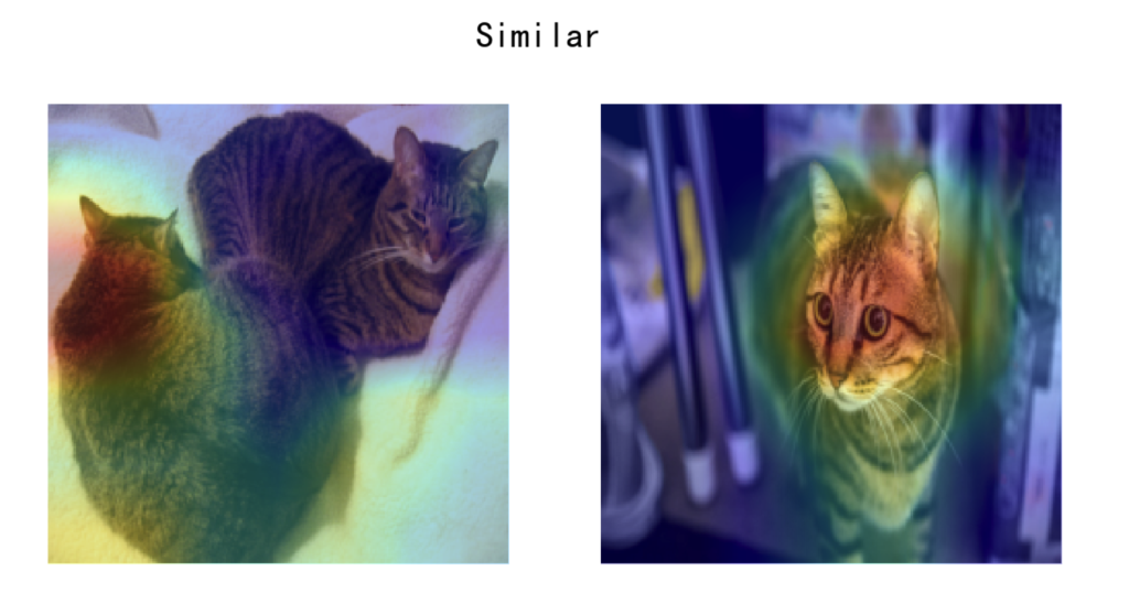
Fig. 2 — Class activation map.

Deployment to TorchServe

Now that we have our trained model for the images of cats, we can easily use TorchServe to serve the model. TorchServe comes with a convenient Command Line Interface (CLI) to deploy locally. It also comes with default handlers for common problems such as image classification, object detection, image segmentation, and text classification. We can always tailor it for our own specifications because TorchServe is open source, which means it is fully extensible to fit any deployment need.

In this section we deploy the PyTorch model to TorchServe. For installation, please refer to the TorchServe GitHub repository. Overall, there are three main steps to use TorchServe:

Archive the model into *.mar.
Start the torchserve process.
Call the API and get the response.

In order to archive the model, three files are needed in our case:

PyTorch encoding model ResNet50 weights encoder_weight.pth.
PyTorch fully connected network weights head_weight.pth.
TorchServe custom handler.

Custom Handler

As shown in /deployment/handler.py, the TorchServe handler accepts data and context. In our example, we define another helper Python class with four instance methods to implement: initialize, preprocess, inference and postprocess.

`initialize`

Initialize works out if GPU resources are available, then identifies the serialized model weights file path and finally instantiates the PyTorch model and puts it to evaluation mode.

 def initialize(self, ctx): """
 load eager mode state_dict based model
 """ properties = ctx.system_properties self.device = torch.device( "cuda:" + str(properties.get("gpu_id")) if torch.cuda.is_available() else "cpu" ) logger.info(f"Device on initialization is: {self.device}") model_dir = properties.get("model_dir") manifest = ctx.manifest serialized_file = manifest["model"]["serializedFile"] model_pt_path = os.path.join(model_dir, serialized_file) if not os.path.isfile(model_pt_path): raise RuntimeError("Missing the model definition file") encoder_reload_weights = torch.load( os.path.join(model_dir, "encoder_weight.pth"), map_location=self.device ) self.encoder_reload.load_state_dict(encoder_reload_weights) self.encoder_reload.to(self.device) self.encoder_reload.eval() head_reload_weights = torch.load( os.path.join(model_dir, "head_weight.pth"), map_location=self.device ) self.head_reload.load_state_dict(head_reload_weights) self.head_reload.to(self.device) self.head_reload.eval() self.initialized = True

`preprocess`

Preprocess reads the image and applies the transformation pipeline to the inference data.

 def preprocess(self, data): """
 Scales and normalizes a PIL image for an U-net model
 """ self.cam_map_left, self.cam_map_right = None, None left_image = data[0]["left"] right_image = data[0]["right"] self.cam = eval(data[0]["cam"]) left_image = Image.open(io.BytesIO(left_image)).convert("RGB") right_image = Image.open(io.BytesIO(right_image)).convert("RGB") left_image = self.image_tfm(left_image)[None, ...] # batch size of 1 right_image = self.image_tfm(right_image)[None, ...] # batch size of 1 return left_image, right_image

`inference`

Inference loads the data to the GPU if available, and passes it through the model consisting of both encoder and fully connected network. If CAM is required, it calculates and returns the heatmap.

 def inference(self, left_image, right_image): """
 Predict the chip stack mask of an image using a trained deep learning model.
 """ if not self.cam: logger.info("no cam") with torch.no_grad(): left_image, right_image = left_image.to(self.device), right_image.to( self.device ) left_embedding = self.encoder_reload(left_image) right_embedding = self.encoder_reload(right_image) res = self.head_reload( torch.cat([left_embedding, right_embedding], dim=1) )[0] else: logger.info("cam") with HookCAMBwd(self.encoder_reload) as hookg: with HookCAM(self.encoder_reload) as hook: left_image, right_image = left_image.to( self.device ), right_image.to(self.device) left_embedding = self.encoder_reload(left_image) right_embedding = self.encoder_reload(right_image) res = self.head_reload( torch.cat([left_embedding, right_embedding], dim=1) )[0] act = hook.stored pred_cls = res.argmax().item() res[pred_cls].backward() grad = hookg.stored self.encoder_reload.zero_grad(), self.head_reload.zero_grad() weight_left = grad[0][0].mean(dim=[1, 2], keepdim=True) self.cam_map_left = (weight_left * act[0][0]).sum(0) weight_right = grad[1][0].mean(dim=[1, 2], keepdim=True) self.cam_map_right = (weight_right * act[1][0]).sum(0) return res

`postprocess`

Postprocess takes the inference raw output which was unloaded from the GPU (if available), and it is then combined with CAM to be returned back to the API trigger.

 def postprocess(self, inference_output): logger.info("start postprocessing") if torch.cuda.is_available(): inference_output = inference_output.cpu() if self.cam: self.cam_map_left = self.cam_map_left.cpu() self.cam_map_right = self.cam_map_right.cpu() if not self.cam: return [inference_output.numpy().tolist()] else: return [ inference_output.detach().numpy().tolist() + self.cam_map_left.detach().numpy().tolist() + self.cam_map_right.detach().numpy().tolist() ]

Now we are ready to set up and launch TorchServe.

TorchServe in Action

Step 1: Archive the Model PyTorch

torch-model-archiver --model-name twin --version 1.0 --serialized-file ./model/encoder_weight.pth --export-path model_store --handler ./deployment/handler.py -f --extra-files ./model/head_weight.pth -f

Step 2: Serve the Model

torchserve --start --ncs --model-store model_store --models twin.mar

Step 3: Call API and Get the Response (here we use httpie).

time http --form POST http://127.0.0.1:8080/predictions/twin left@sample/c1.jpg right@sample/c2.jpg cam=False
>>>
HTTP/1.1 200
Cache-Control: no-cache; no-store, must-revalidate, private
Expires: Thu, 01 Jan 1970 00:00:00 UTC
Pragma: no-cache
connection: keep-alive
content-length: 46
x-request-id: e51e2f15-a9b6-4522-b700-c0f5e35008a7 \[ -0.938737690448761, 0.7865392565727234
\] real 0m1.765s
user 0m0.334s
sys 0m0.036s

The first call has longer latency due to model weights loading defined in initialize, but this will be mitigated from the second call onward. For more details about TorchServe setup and usage, please refer to notebook/02_pytorch_inference.ipynb [link].

Deployment to Amazon SageMaker Inference Endpoint

For customised machine learning model deployment and hosting, Amazon SageMaker is fully modular, which means we can always bring in customised algorithms and containers and use only the services that are required. In our case it is the Amazon SageMaker model and endpoint. Specifically, we are building a TorchServe container and hosting it using Amazon SageMaker for a fully managed model hosting and elastic-scaling experience, with simply a few lines of code. On the client side, we get predictions with simple API calls to its secure endpoint backed by TorchServe.

There are four steps to set up a SageMaker endpoint with TorchServe:

Build a customized Docker image and push to Amazon Elastic Container Registry (Amazon ECR). The dockerfile is provided in root of this code repository, which helps setup CUDA and TorchServe dependencies.
Compress *.mar into *.tar.gz and upload to Amazon Simple Storage Service (Amazon S3).
Create SageMaker model using the Docker image from step 1 and the compressed model weights from step 2.
Create the SageMaker endpoint using the model from step three.

The details of these steps are described in notebook/03_SageMaker.ipynb [link]. Once ready, we can invoke the SageMaker endpoint with images in real-time.

Real-time Inference with Python SDK

Read the sample images.

cam = False
r = requests.Request( "POST", "http://localhost:8080/invocations", files={ "left": open("./sample/c1.jpg", "rb"), "right": open("./sample/c2.jpg", "rb"), }, data={"cam": str(cam)}
)
r = r.prepare()
content_type = r.headers["Content-Type"]
payload = r.body
content_type, type(payload)

Invoke the SageMaker endpoint with the image and obtain the response from the API.

client = boto3.client("sagemaker-runtime")
response = client.invoke_endpoint( EndpointName=endpoint_name, ContentType=content_type, Body=payload )
res = response["Body"].read()
neg, pos, *maps = eval(res)
neg, pos
>>> (-0.9403411149978638, 0.7890562415122986)

Web Application Demonstration

Streamlit is an open source framework for data scientists to efficiently create interactive web-based data applications in pure Python. It allows for quick end-to-end deployment with minimal effort and the ability to scale out the application as needed in a secure and robust way, without getting bogged down in time-consuming, front-end development.

To run the Streamlit application provided in the root of this code repository, first install the dependencies:

pip install -r requirements-demo.txt

And setup the AWS credentials according to Set up AWS Credentials and Region for Development documentation. After updating SAGEMAKER_ENDPOINTS and REGIONS in the ./app.py according to your setup, run:

streamlit run app.py

This will enable users to upload images, invoke the SageMaker endpoint, and visualise the inference results with model explainability.

Clean up

Make sure that you delete the following resources to prevent any additional charges:

Amazon SageMaker endpoint.
Amazon SageMaker endpoint configuration.
Amazon SageMaker model.
Amazon Elastic Container Registry (Amazon ECR).
Amazon Simple Storage Service (Amazon S3) Buckets.

Conclusion

This repository presents an end-to-end workflow for training a Twin Neural Network with PyTorch and Fast.ai, followed by its deployment with TorchServe eager mode on Amazon SageMaker endpoint. You can use this repository as a template to develop and deploy your own deep learning solutions. We then used an application built with the open source Streamlit framework that demonstrates how end users can use the new model to compare two images and visualise the results. This approach eliminates the self-maintenance effort to build and manage a customised inference server, which helps to speed up the process from training a cutting-edge deep learning model to its online application in the real world, at scale.

Reference

CategoryNews

Tagsamazon-sagemaker artificial intelligence Cloud Computing deep learning deployment fastai image-classification machine learning natural language processing neural-networks neural-networks-applications Predictive Modeling pytorch recommendation-system torchserve training